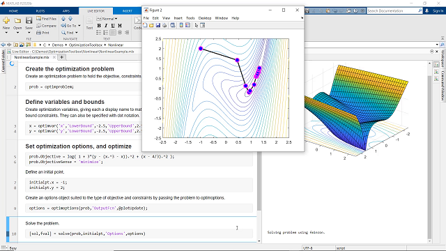
Optimization and numerical analysis are essential techniques in various fields, including engineering, economics, finance, and scientific research. MATLAB, with its powerful numerical computing capabilities and extensive optimization toolboxes, provides a versatile platform for performing optimization tasks and numerical analysis. In this comprehensive guide, we will delve into the world of optimization and numerical analysis in MATLAB, covering everything from solving mathematical equations to optimizing complex systems and algorithms.
Table of Contents
- Introduction to Optimization and Numerical Analysis
- Solving Equations and Systems of Equations
- Minimization and Maximization Problems
- Optimization with Constraints
- Nonlinear Optimization Techniques
- Global Optimization Methods
- Numerical Integration and Differentiation
- Curve Fitting and Interpolation
- Eigenvalue and Eigenvector Computations
- Linear and Nonlinear Least Squares Problems
- Partial Differential Equations (PDEs) Solvers
- Applications in Engineering and Scientific Research
- Best Practices and Tips
- Conclusion
1. Introduction to Optimization and Numerical Analysis
Optimization involves finding the best solution to a problem from a set of possible solutions, often subject to constraints. Numerical analysis, on the other hand, focuses on solving mathematical problems using numerical methods and algorithms. Both optimization and numerical analysis play a crucial role in various applications, including engineering design, financial modeling, and scientific simulations.
2. Solving Equations and Systems of Equations
MATLAB provides functions for solving both linear and nonlinear equations, as well as systems of equations. Users can employ methods such as Newton-Raphson iteration, bisection method, and secant method for solving equations numerically.
% Example of solving a nonlinear equation

fun = @(x) x^2 - 3*x + 2;

x = fzero(fun, 0);
3. Minimization and Maximization Problems
Minimization and maximization problems involve finding the minimum or maximum value of a function, respectively. MATLAB offers optimization functions such as fmincon, fminunc, and fminsearch for solving such problems.
% Example of minimizing a function

fun = @(x) x^2 - 3*x + 2;

x = fminunc(fun, 0);
4. Optimization with Constraints
In many real-world optimization problems, constraints must be satisfied while optimizing the objective function. MATLAB’s optimization toolbox provides functions for constrained optimization, allowing users to specify both equality and inequality constraints.
% Example of constrained optimization

fun = @(x) x(1)^2 + x(2)^2;

x0 = [0, 0];

A = [1, 1];

b = 1;

x = fmincon(fun, x0, A, b);
5. Nonlinear Optimization Techniques
Nonlinear optimization involves optimizing nonlinear objective functions subject to constraints. MATLAB offers a range of algorithms for nonlinear optimization, including gradient-based methods, genetic algorithms, and simulated annealing.
% Example of nonlinear optimization with a genetic algorithm

fun = @(x) x(1)^2 + x(2)^2;

nvars = 2;

options = optimoptions('ga', 'PlotFcn', @gaplotbestf);

[x, fval] = ga(fun, nvars, [], [], [], [], [], [], [], options);
6. Global Optimization Methods
Global optimization aims to find the global minimum or maximum of a function over a specified domain. MATLAB provides global optimization functions such as ga, patternsearch, and globalSearch for solving global optimization problems efficiently.
% Example of global optimization with pattern search

fun = @(x) x^2 - 3*x + 2;

x = patternsearch(fun, 0);
7. Numerical Integration and Differentiation
Numerical integration involves approximating the integral of a function over a specified interval, while numerical differentiation involves approximating the derivative of a function at a point. MATLAB provides functions such as trapz, quad, and diff for numerical integration and differentiation.
% Example of numerical integration

x = linspace(0, 1, 100);

y = sin(x);

integral_value = trapz(x, y);
8. Curve Fitting and Interpolation
Curve fitting involves finding a function that best fits a given set of data points, while interpolation involves estimating values between known data points. MATLAB’s curve fitting toolbox offers functions for fitting curves to data using linear and nonlinear regression techniques.
% Example of curve fitting

x = 1:10;

y = 2*x + randn(1, 10);

fit_result = fit(x', y', 'poly1');
9. Eigenvalue and Eigenvector Computations
Eigenvalue and eigenvector computations are essential in various mathematical and scientific applications, including structural analysis, quantum mechanics, and data analysis. MATLAB provides functions such as eig and svd for computing eigenvalues and eigenvectors of matrices.
% Example of eigenvalue computation

A = [1, 2; 3, 4];

[eig_vectors, eig_values] = eig(A);
10. Linear and Nonlinear Least Squares Problems
Least squares problems involve minimizing the sum of the squares of the differences between observed and predicted values. MATLAB offers functions such as lsqnonlin and lsqcurvefit for solving linear and nonlinear least squares problems.
% Example of linear least squares fitting

x = 1:10;

y = 2*x + randn(1, 10);

fun = @(c, x) c*x;

c = lsqcurvefit(fun, 1, x, y);
11. Partial Differential Equations (PDEs) Solvers
Partial differential equations (PDEs) arise in many areas of science and engineering, describing the behavior of systems involving multiple variables. MATLAB provides functions such as pdepe and pdeint for solving initial-boundary value problems (IBVPs) and partial differential equations numerically.
% Example of solving a PDE numerically
12. Applications in Engineering and Scientific Research
Optimization and numerical analysis have numerous applications in engineering, scientific research, finance, and other fields. MATLAB’s optimization and numerical analysis capabilities are widely used in areas such as structural optimization, parameter estimation, computational fluid dynamics, and image processing.
% Example of application in engineering
13. Best Practices and Tips
To ensure successful optimization and numerical analysis in MATLAB, it is essential to follow best practices such as:
- Choosing the appropriate optimization algorithm for the problem at hand.
- Checking convergence criteria and adjusting solver parameters accordingly.
- Validating results against analytical solutions or experimental data.
- Utilizing vectorized operations and parallel computing for improved performance.
- Documenting code and results for reproducibility and collaboration.
14. Conclusion
Optimization and numerical analysis are fundamental techniques for solving complex mathematical problems and optimizing systems in various domains. MATLAB’s optimization toolbox and numerical computing capabilities provide powerful tools for tackling optimization problems, solving equations, and performing numerical analysis efficiently.